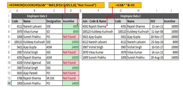
Sometime you need to apply VLookup with multiple criteria to get the result. If you want to use VLookup with two lookup values and also remove error results then you have to use IFError function along with VLookup function.
VLookup with IFError function
This tutorial shows you how could you easily VLookup multiple values in Excel which is based on one or more conditions. If you have two tables and want to check multiple columns criteria in another table and want to get matched column value in first table. In that situation you must have to use VLookup function in active worksheet along with IFError function.
IFError function allows you to remove any error value with an expression as per your need. But before start to know how to use VLookup with two lookup values using IFError function, you have to know about the VLookup and IFError function in Excel.
VLookup Function in Excel
VLookup function is used to search a value in the first column of a table_array or range of cells. After that return corresponding value in the same row and from a column that you specify. First column is always sorted in the ascending order. VLookup stands for Vertical Lookup. This function is located in the “Lookup and Reference” category in Microsoft Excel.
VLookup (lookup_value, table_array, col_index_num, [range])
Lookup_value: Lookup value is the value to be searched in the extreme first column of the table array.
Must Read: Excel VLookup Find First, 2nd Or Nth Match Value in Excel?
Table_array: Table array have two or more columns of data. Give cell reference of a range or range name.
Col_index_num: The column index_number in the table from which the searched value must be returned.
If col_index_num of returns 1 then the value in the first column in table_array. If it is less than or greater than 1, this function returns an error value #VALUE!. or #REF! respectively.
Range_lookup: It is an options part of this function. There are two options available in this part.
TRUE: Appropriate Match: This option work properly when first column of your table will be sorted in ascending order only otherwise it displays wrong
result.
False: Exact Match: VLookup by default check only on exact match method.
IFError function in Excel
IFError function allows you to return an expression when your formula generates an error. If you don’t want to show any error in any cell during applying the formula then you have to use IFError function in active sheet. You can use IFError function to trap and handle different types of errors in a formula.
IFError (value,value_if_error)
Must Read: Advanced VLookup trick with Data Validation in Excel
Value: This argument is used to check for an error. It may be the value or reference or formula.
value_if_error: If any error is evaluated after applying the formula, then use given argument.
For e.g. If you have two table of employees data in active worksheet and want to get the incentive amount of employees which match the code and name. You have to take given simple steps to get the result as per given criteria.
VLookup with Two Lookup Values using IFError function
You have to take following steps to apply VLookup function to lookup two values.

Step 1: You have to join emp code and name in employee data 2 table with the help of ampersand operator. To join emp code and name you have to type given formula in cell F3 =G3&” “& H3. Now drag this formula for rest of the cells.
Step 2: To view employee incentive in employee data 1 table you have to type given function in cell D3.
=VLOOKUP(A3&” “&B3,$F$2:$J$9,5,0). Drag this formula for rest of the cell you can check few cells shows an error. If you don’t want to keep errors then you have to use IFError function in the function. =IFERROR(VLOOKUP(A3&” “&B3,$F$2:$J$9,5,0),”Not Found”).
Now when you drag this function for rest of the cells all error values removed from all those cells which code and name not matched with given condition.
I hope you like this VLookup with Two Lookup Values using IFError function guide. If you want to highlight all those cell which code in not found then you have to use conditional formatting in active worksheet. Conditional formatting allows you to apply different kind of formats on selected cell or range of cells as per requirement.