Goal Seek is an important utility of Microsoft Excel. It is an important part of What-If-Analysis, which allows you how to one value in the formula impacts to all of the other values. Goal Seek is the best tool used to find the result by adjusting an input value. In this article we have to discuss how to use Goal Seek feature in Microsoft Excel. Goal Seek is an important feature of What-If-Analysis. There are lot of situation in which you have to use Goal Seek feature in Microsoft Excel.
Goal Seek feature used to change the single value and view the impact for other values. It is an important part of What-If-analysis. You can change the single value and view the impact on the resulted value. Goal Seek feature allows you to change single variable value while solver allows you to change more than one variable values and view the impact for others. Data tables also an important part of What-If-Analysis. You can not create the one input data table but also create two input data table in MS Excel.
In this article we try to tell you few easy steps which helps you to use Goal Seek in Microsoft Excel. If you want to take money as a loan and want to know how much amount you have to pay against the loan, what is the interest rate for particular duration of loan. With the help of Goal Seek you can easily calculate the interest rate against the loan amount.
Must Read: How to remove spaces from text string in Excel
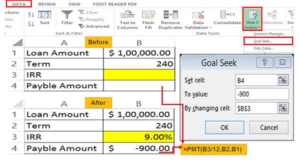
For eg: If you want to borrow $100000/- for the duration of 240 months. You have already decide to pay up to $900 in each month as a instalment against the loan. Now you want to know what is the final interest rate against this loan.

How to use Goal Seek feature in Microsoft Excel
Step 1: Create a new or blank worksheet.
Step 2: Type the given formula in cell B4 =PMT(B3/12,B2,B1) to calculate the instalment amount against the loan. PMT is an important financial function which is used to calculate the loan amount. PMT stands for payment monthly instalment.
Step 3: Select the cell B4 and click on the Data tab > Click on the What-If-Analysis command > Click on the “Goal Seek” option.
Must Read: Prevent duplicate values with Data Validation in MS Excel
Step 4: In the Set cell box, type of click on the cell B4.
In the To Value box, type -900 and By changing cell box, type or click on the $B$3. Now click on the OK button to get the result.
Finally you have to press OK button. The Goal Seek command displays the final interest rate against the loan amount. I hope after reading this guide you can easily use Goal Seek in Microsoft Excel. If you have any query regarding this article please write us in the comment box. Thanks to all.