Pivot table is an important feature of Excel, which allows you to manage and summarize your large worksheet data. In this article, we will discuss how to show report filter pages Excel pivot table data. You can use, Pivot table which is an important and useful tool used for data analysis purpose in Excel.
Must Read: How to create and modify calculated fields in Pivot Table
Before doing this job you must have to know how to do grouping and grouping of pivot table data in excel for analysis purpose. Grouping data in a PivotTable helps you to show a subset of data to analysis. You can easily group row wise or columns wise pivot table data in excel. You can start grouping into Seconds, Minutes, Hours, Days, Months, Quarters and Years.
Steps to do Grouping of Excel Pivot Table Data
In an active pivot table you have to follow given simple steps to start grouping of pivot table data.
Steps 1: Click a cell in the first column of active pivot table. Click on the “Analyze” tab in Pivot Table Tools menu.
Step 2: In the ribbon bar, click on the “Group Selection” option or the button “Group Field” in the toolbar. You can also right click on active cell in pivot table and choose “Group…” option.
Step 3: In Grouping window starting and ending date will appear automatically. You can also change start and end data as per your requirement.
Must Read: How to Show Percentage of Parent Total in an Excel PivotTable
Step 4: In By section you must have to choose the criteria which is used for grouping purpose. Here you can choose any required groping criteria as per your need. In this guide we have to we will choose the “Years”option for grouping. Finally, click on the OK button in the “Group” window. You can check as per choosing option result is shown in the active pivot table.
Steps to do Grouping Data of Excel Pivot Table Data
If you don’t want to keep grouping of pivot table data, then you have to follow given steps to grouping of pivot data.
Click on any active column in the pivot table. If you remove all the grouping from active pivot table then click “Ungroup” option. You can choose ungroup option either from choose right mouse button or click on the “Ungroup” option in Analyze menu.
How to Show Report Filter Pages Excel Pivot Table Data
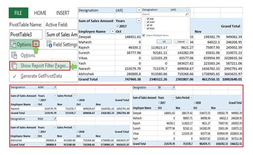
There is one many hidden feature of pivot tables which save your time during working on large worksheet data in Excel. After finish the grouping process of your pivot data, you can easily generate separate filter reports. Excel Pivot Table allows you to show the items within the Report Filter on different separate worksheets within your active workbook. To do this job take given following steps.

Step 1: Open your Pivot Table from which you want to view filter pages report from active pivot data.
Must Read: How to Find Duplicates with Pivot Table in Excel
Step 2: Choose Pivot Table Tools > Analyze > Click on the “Options” drop down arrow in PivotTable group section. Click on the “Show Report Filter Pages...” option.
Step 3: In Show Show Report Filter Pages dialog box, you can check all the generated pages are based on the “Designation” filed. You just click on the OK button. Now, you can check there are three separate report filter pages generated with the name of RSM, ASM and SR.
I hope you like this guide, please if you have any query and any suggestion then tell us. We try to best for resolve your query. Thanks.