During working on an Excel you have to apply different functions on any worksheets which have the same body structure. But you have to face difficulty to calculate the accurate result. In this guide we have to discuss how to apply formula on multiple worksheets with 3D reference in Excel.
3D reference is an unique technique which is very useful for all users who are working on Excel to prepare different MIS reports. If you have more than one worksheet which have same the body structure and want to apply same function on these sheets then you have to face problem. But after reading this guide you can easily get an idea apply formula on multiple worksheets with 3D reference in Excel.
Must Read: How to find duplicates using conditional formatting in Excel
How to Apply formula on multiple worksheets with 3D reference in Excel
Most of the Excel users does not aware about this trick. But it is an interesting and useful trick which helps you to solve your different problems. If you want to apply any function or formula on different sheets and want to view the result on any another sheet, then you have to face problem. But after reading this guide you can easily apply formula on multiple worksheets with 3D reference in Excel.
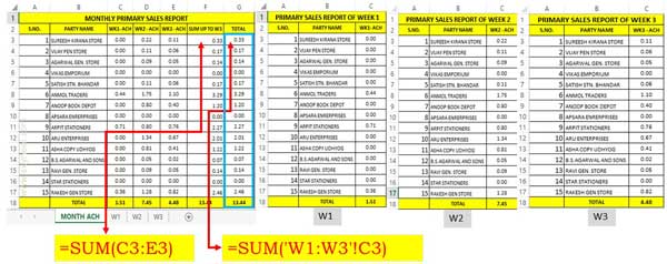
For eg. If you have three seprate worksheet’s in which you have weekly achievements which have same body structure & number of records. Now, you want to calculate the total of all weekly achievements of all different sheet’s values in another separate sheet. In that situation you have to take few given simple steps to apply formula on multiple worksheets with 3D reference in Excel.

Step 1: Open an existing worksheet or create a workbook in which have different records with same body structure. For eg. W1, W2, W3.
Must Read: How to Search Duplicate Values with VLookup function
Step 2: Now take cursor on cell G3 in “Month ACH” worksheet and apply given formula. You can either type manually this formula or you can also select cell C3 in W1 and hold on the Shift key and click on the last W3 sheet tab.
=SUM(‘W1:W3’!C3)
Step 3: After doing this to finish the formula press enter key to get the result. Now drag this formula to rest of the cells to get the result. You can also press Ctrl+D shortcut key to get quick result.
I hope after reading this guide most of the excel users problem will be solved. Now you can easily apply function on multiple worksheets with 3D reference in Excel. If you have any suggestion regarding this guide then please write us in the comment box. Thanks to all.