Hi guys we know very well about the importance of MS Excel in our life. Without the Excel we are not able to prepare of MIS Reports, Data Sheet, Employee records and many more. Today we discuss about the most important utility Data Validation and VLookup Function in MS Excel. We know that both of these are important and most useful part of MS Excel.
Lot of time we need to use “Data Validation” and “VLookup” function in same worksheet to view the required result. Today, we know how to Use Data Validation for prepare drop down lists for Names of employees, product list and others things and also search and watch the Price in another column with the help of using VLookup function in MS Excel. So, today in this article we have to discuss how to use Data Validation for naming the range and VLookup Function in MS Excel.
Data Validation: This command is used to prevent invalid data being entered into the cell. It is used for naming the range of selected cell contents, create drop down list, apply restriction as per your need on selected cells and many more.
VLookup Function: VLookup function in MS Excel is used to looks for a value in the left most column of a table, and then return a value in the same row from a column you specify.
Must Read: How to Restrictions on Columns by Data Validation in Excel
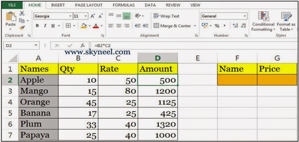
In this example, we have to prepare a sheet in which create list using data validation and then apply VLookup formula to search amount as per selected fruit name in the list:
How to use Data Validation and VLookup Function in MS Excel
Step 1: Create the following table in MS Excel.
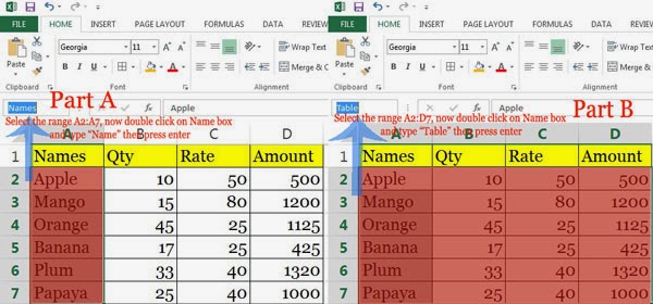
Step 2: To set the name of a range, select the range “A2:A7” >> Click Name box >>> Type the name of selected range like “Names”, then press enter.
Step 3: To set the name of another range, select the range “A2:D7” >>>Click Name box >>>Type the range name of selected range like “Table” then press enter.
Note: When you click name box in active window of excel sheet and select Name it automatically select range A2:A7.
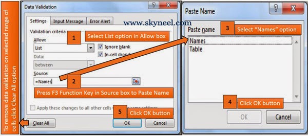
Step 4: Select the Cell F2 >>> Press ALT+D+L (To directly open Data Validation dialog box) or You can also click Data Tab >>> Data Validation >>> Data Validation >>> Select “List” option in Allow >> Press F3 in Source Box and select “Names” then click OK button >>> Click OK button in Data Validation dialog box.
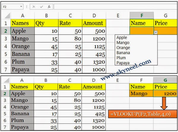
Step 5: Type following formula to display amount in Cell G2 as per choosing Name of fruit in Cell F2 using VLookup formula =VLOOKUP (F2,Table,4,0) then press enter.
Note: During type of VLookup formula press F3 function key to insert Table option.
Step 6: When you choosing any fruit name in Cell F2, Excel automatically displays his amount in Cell G2.
Must Read: How to Use Decimal Option in Data Validation in Excel
I hope you like this Data Validation and VLookup Function guide. after reading this article you will be able to easily use Data Validation and VLookup Function in MS Excel. Kindly share your knowledge with others and send your important suggestions in the comment box regarding this article. Thanks to all of you.


