Sometime it is necessary to “Switching” or “Transposing” the orientation of data from row to column-wise or column to row-wise to make it easier for more understanding, presentable and effective by using Transpose option in MS Excel. I have an easiest example from which you can easily change orientation of your data. How to Switch or Transpose Row And Column Data in easy way. The transpose option is used to convert rows copied data into columns and columns copied data into rows.
Methods of Data Transpose (Switch or Transpose Row And Column Data) in Excel:
1. By Using Paste Special -> Transpose2. By Using Transpose Function in Lookup & Reference category.
Must Read: Use Data Validation, Naming the range and VLookup Function
First Method by Transpose Option
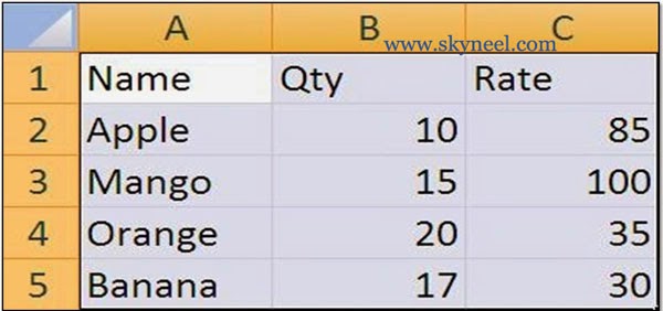
Step 1: Select the range A1:C5 which you want to transpose. (Before Transpose)
Step 2: Press Ctrl + C or you can also click Copy button in Home Tab.
Step 3: Take cursor on new location in which you want to view the result. For Example: F1
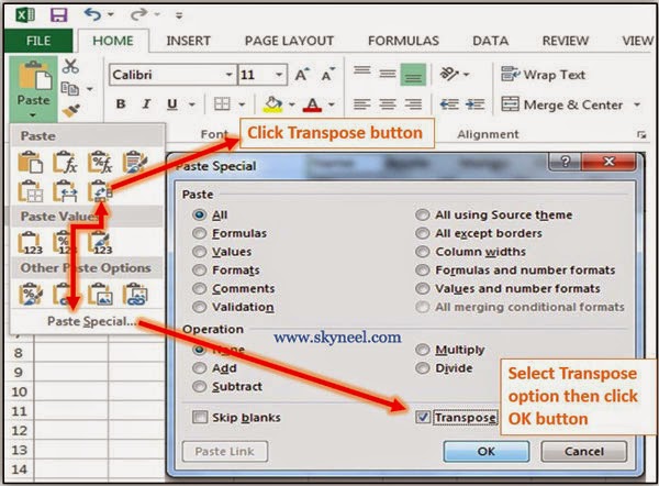
Step 4: Click Paste button -> Click Transpose button or you can also select Transpose option in Paste Special dialog box.
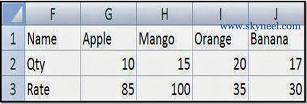
Step 5: After choosing this option range (F1:J3) covert into rows to column wise and column to row wise data like this. (After Transpose)
Second Method by Transpose Function
You can also use Transpose function from Lookup and Reference category in Formula Tab. The TRANSPOSE function is also used to convert rows copied data into columns and columns copied data into rows.
Must Read: MS Excel : Vlookup Function with a Spreadsheet
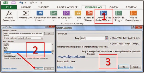
Syntax of TRANSPOSE function: = TRANSPOSE (array) array – It is a range of cells or values which you want to transpose. You have to take following steps to use this function
Step 1: Select the range F1:J3
Step 2: Click Formula >>> Lookup & Reference >>> Select Transpose Function Step 3: Select the range A1:C5 in Array box then press Ctrl + Shift + Enter Key
Step 4: The data of range A1:C5 transpose and shows in cells F1:J3.
I hope you like this Switch or Transpose Row And Column Data guide from which you will be able to easily Switch or Transpose Row And Column Data without any extra efforts. If feel any problem in this guide then please use comment box. Thanks to all.


