Most of the person don’t known about the reverse VLookup in Excel. All we know very well VLookup is an important lookup function which search the value from left to right in given array or table. But sometime you need to lookup the value in reverse order that means right to left. It is not so easy to search the required value in reverse order. But there is no need to worry this guide helps you to know how to use reverse VLookup in Excel with the VLookup function.
All we know very well that VLookup is one of the most important functions of Excel. VLookup function is found in Lookup and Reference category. This function used to lookup a value in the left most column of a table, and then return a value in the same row from a column you specify. You can use VLookup function in searching duplicate values, hide error, search value with multiple criteria and many more. You can use VLookup function with the combination of Data Validation, IFNA, Match, and other function.
Must Read: How to use Countif function with wildcards in Excel
Syntax of VLookup function in Excel
The Microsoft Excel VLookup function is used to search specific value in the extreme left column of the table_array. It provides the value in the same row which is based on the index number.
VLookup (lookup_value, table_array, col_index_num, [range])
Note: VLookup function is used to search the value of extreme left column. So, you have to arrange first column of any table or array in ascending order, otherwise VLookup function is not able to provide the accurate result.
Lookup_value: The value to be searched in the extreme first column of the table array.
Table_array: Two or more columns of data. Give cell reference of a range / range name.
Col_index_num: The column index_number in the table from which the searched value must be returned.
Range_lookup: It is an options part of this function. There are two options available in this part.
TRUE: Appropriate Match: This option work properly when first column of your table will be sorted in ascending order only otherwise it displays wrong
result.
False: Exact Match: VLookup by default check only on exact match method.
Choose Function in Excel
Choose function allows you to choose a value or action to perform from a list of values which is based on an given index number.
Syntax of Choose Function:
Choose(index_num, value1, [value2], …)
Index_num: It is required number which specifies the value argument is selected. It may contain numbers, cell reference or formula between 1 to 254.
If index_num is 1, CHOOSE returns value1; if it is 2, CHOOSE returns value2; and so on.
If index_num is less than 1 or greater than the number of the last value in the list, CHOOSE returns the #VALUE! error value.
If index_num is a fraction, it is truncated to the lowest integer before being used.
Value1, value2, … Value 1 is required, subsequent values are optional. 1 to 254 value arguments from which CHOOSE selects a value or an action to perform based on index_num. The arguments can be numbers, cell references, defined names, formulas, functions, or text.
Must Read: Latest 7 Excel Tricks which makes you an Excel Expert
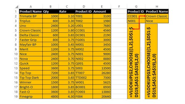
For Eg: If you have Product name, Qty, Rate, Product ID and Amount in a worksheet. Now you want to lookup and product name which is based on Product ID. In that situation you must have to use backwards VLookup in Excel to search in Reverse order. You can take help of VLookup and Choose function to get the correct result.
How to use Reverse VLookup in Excel with VLookup Function
You must have to take given simple steps to reverse VLookup in Excel using VLookup function.

Step 1: Fill the given required detail in any blank worksheet to use reverse VLookup in Excel with VLookup function.
Step 2: Place the Cursor on Cell H2 in which you want to apply the given formula. After applying the formula you will get the Product name in Cell G2.
=VLOOKUP(G2,CHOOSE({1,2},$D$1:$D$19,$A$1:$A$19),2,0).
You can check VLookup and Choose functions to get the correct result. When you change the Product ID, the Product name is automatically change with the help of reverse VLookup function in Excel.
I hope after reading this guide you can easily understand how to use backwards VLookup in Excel to search the value in Reverse order. If you have any suggestion regarding this guide then please write us in the comment box. Thanks to all.