Hi, today we are talking on Index and Match most popular and powerful function in Microsoft Excel. You can use index match function in excel separately or with combination of other functions as per your need. In this guide we have to discuss how to use index and match functions for advanced lookup in Excel. Index and Match and VLookup functions found in the Lookup and Reference category.
These functions allows you to quickly lookup the values in the given table or array and return the result which match the condition. When you are facing the interview or preparing the MIS reports in that situation these functions are too much important for us. Most of the person like to use index match function at the place of VLookup function in active worksheet.
How to use index and match functions for advanced lookup in Excel
Before start how to use index and match functions for advanced lookup in Excel, you must know about them. Let’s start discuss about these functions.

Index Function in Excel
Index function return a value or the reference number to a value from given range of cells or table array.
Must Read: How to use COUNTIFS and SUMIF together in Excel
INDEX(array, row_num, [column_num])
Array : It is a range of cells or an array constant.
Row_num : Selects the row number in an array from which to return a value. If Row_num is omitted, Column_num is required.
Column_num : It is an optional. Selects the column number in an array from which to return a value. If Column_num is omitted, Row_num is required.
Match Function in Excel
This function is used to returns the relative position of an item in the given array or range of cells that match a specific value in specific order.
MATCH (lookup value, lookup array, [match_type] )
lookup_value: The value that you want to match in lookup_array. The lookup_value argument can be any number, text, logical value or a cell reference to a number, text, or logical value.
lookup_array: It is range of cells being searched.
match_type: It is an optional. The number -1, 0, or 1. The match_type argument specifies how Excel matches lookup_value with values in lookup_array. By default value for this argument is 1.
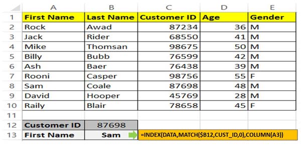
Step 1: Create the following worksheet to use index and match functions for advanced lookup in Excel.
Must Read: How to Find Duplicates with Pivot Table in Excel
Step 2: Select the range from A2:E10 and click on the name box and set the range name like “Data”. Just like this select the range C2:C10 and set the range name “CUST_ID” with the help of name box.
Step 3: Fill the customer id in the cell B12 to find out customer name which you want to find in your active database.
Step 4: Type the following given formula in cell B13 =INDEX(DATA,MATCH($B12,CUST_ID,0),COLUMN(A3)) and press enter to view the result.
Now, you can use index and match functions for advanced lookup in Excel. If you have any suggestion regarding this guide then please write us in the comment box. Thanks to all.