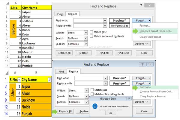
You can easily apply bold font character formatting in Excel, but you have to face lot of issue when you try to filter bold cells only. In this guide we have to discuss an easy trick which allows you to filter bold cells character formatting in Excel.
Lot of peoples have to face this type of situation and they have no choice how to deal with this situation. If you have a huge set of data and want to filter only highlighted bold cells on which apply character formatting in Excel. If you want to use filter command to do this job, then there is no choice. You have to waste lot of time to get the proper result.
Must Read: Lock or Unlock particular areas of a protect worksheet in Excel
How to Filter Bold Cells Character Formatting in Excel
If you want to filter bold cells character formatting in Excel with the help of Find and Replace command. All we know Find command is used to find the specific characters or words. You can use Replace command to find and replace the characters as as per your need. Now, you have to take given steps which helps you to filter bold cells character in Excel.

Step 1: First you have to create a worksheet.
Step 2: Open Find and Replace dialog box by pressing Ctrl+H shortcut key or click Home > Find & Select > Replace.
Step 3: By default there is “No Format Set” option is already set at Find what box. Now, Click on the Choose Format From Cell… and choose formatted cell in-front of Find what box. You can check there is “Preview*” is shown at the place of “No Format Set”.
Must Read: How to quickly remove all blank cells in MS Excel
Step 4: Click on the Format button and set the required formatting by clicking on the Format option in front of Replace with box.
Step 5: Click on the Replace All button. Formatting applied on all those cells which have character formatting. Now select the complete range of cells and turn on filter option.
Step 6: Click on the Filter by color option and select the formatted color.
I hope after reading this guide you can easily filter bold cells character in Excel. If you have any suggestion regarding this guide then please write us in the comment box. Thanks to all.