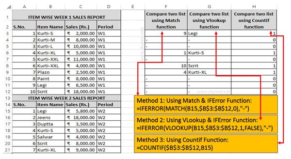
During working on Excel you want to check if any particular data of one column matched with another column data or not ? You can easily compare two list data in Excel using few simple tricks. In this guide we have to discuss how to compare data between two lists in Excel.
If you have one or more same kind of data then you can easily compare two columns in Excel for find the matches and differences. Most of the users need to compare two columns in excel sheets. If you do this job manually then you will take lot of time. If you don’t have enough time and want to compare data between two lists in Excel sheet then you have to use given methods.
How to compare data between two lists in Excel
During working in active worksheet if you have two columns or list and want to compare them then you have to use given methods. Excel has different functions which allows you to quickly compare two columns data in Excel. These functions not only user friendly but also take little bit time for comparison.
- How to Identifying Duplicate Values in two Excel worksheets
- 3 Ways to find duplicate values on same worksheet – Excel

Method 1: Compare data between two lists in Excel – Using Match & ISError Function
ISError Function in Excel
It is a built-in function in Excel. ISError function is used to checks whether a value is an error (#N/A, #VALUE!,#REF!, #DIV/0!, #NUM!, #NAME?, or #NULL!) and returns True or False.
Syntax of ISERROR: ISERROR (Value)
Value: It is the value you want to test. Value can refer to a cell, formula or a name that refers to a cell, formula or value.
Match Function in Excel
Match function is used to search specific value in the active worksheet. Now this function return the exact position of the value in the given range.
Syntax of Match: MATCH(lookup_value, lookup_array, [match_type])
lookup_value: Lookup values is the value which is search in the table array.
lookup_array: It is the range of cells in which you have to search lookup_value.
match_type: It’s an optional. The default value is 1. The number -1, 0, or 1.
1: Used to find the largest value that is less than or equal to lookup_value.
2: Used to find the first value that is exactly same to lookup_value.
-1: Used to find the smallest value that is greater than or equal to lookup_value.
Step 1: Fill the given required information in active worksheets to start the comparison data between two columns in Excel.
Step 2: Type the following given formula in cell F3 =IFERROR(MATCH(B15,$B$3:$B$12,0),”-“) and press enter to view the result.
Step 3: Select the cell F3 and drag the formula with the help of fill handle from F3:F12.
Method 2: Compare data between two columns in Excel – Using VLookup Function
VLookup is an important lookup function which is found in Lookup & Reference category. VLookup allows you to searches a value in the extreme left column of the table_array and provides the value in the same row which is based on the index number.
Syntax of VLookup function: VLookup (lookup_value, table_array, col_index_num, [range])
Note: Before using the VLookup function, first you need to arrange first column of a table or array in the ascending order, otherwise VLookup function is not able to provide the accurate result.
Lookup_value: The value to be searched in the extreme first column of the table array.
Table_array: Two or more columns of data. Give cell reference of a range / range name.
Col_index_num: The column index_number in the table from which the searched value must be returned.
If col_index_num of returns 1 the value in the first column in table_array. If col_index_num is: Less than 1, this function returns an error value the #VALUE!. Sometime it is a greater than the number of columns in table_array, this function returns error value #REF!.
Range_lookup: It is an options part of this function. There are two options available in this part.
TRUE: Appropriate Match: This option work properly when first column of your table will be sorted in ascending order only otherwise it displays wrong
result.
False: Exact Match: VLookup by default check only on exact match method.
Step 1: Type the following given formula in cell G3 =IFERROR(VLOOKUP(B15,$B$3:$B$12,1,FALSE),”-“) and press enter to view the result.
Step 2: Select the cell G3 and drag the formula with the help of fill handle from G3:G12.
Method 3: Comparison data between two columns in Excel – Using Countif Function
Countif is an important function of Excel. You can easily count all those cells that meet the criteria from given cells values in any worksheet.
Syntax of Countif function: COUNTIF (range, criteria)
range: It is the range of continuous cells which you want to evaluated for the specific condition.
criteria: It is the condition in the form of any number, expression or text value that define which cells to be counted.
Step 1: Type the following given formula in cell H3 =COUNTIF($B$3:$B$12,B15) and press enter to view the result.
Step 2: Select the cell H3 and drag the formula with the help of fill handle from H3:H12.
I hope after reading this guide you can choose any method to compare data between two lists in Excel sheet. All these methods allows you to quickly compare two columns in Excel sheet. If you have any suggestion regarding this guide then please write us your suggestion in the comment box. Thanks to all.