Hi, everyone at present time most of the person’s know about very well about the MS Excel. MS Excel is an electronic spreadsheet application software which is used for data analysis, modelling, representing numerical data in term of chart, provide quick results of complex calculations using different commands and functions. Today we discuss another very important topic how to combine IF with VLookup function to hide any type of errors in active sheet in MS Excel.
This question is faced by lot of persons when they go for interview for the job in any company or facing the questions about the which is related to “VLookup” function during the interview session. You know very well “VLookup” is one of the most important functions which are found in “Lookup and Reference” category of Microsoft Excel. There are lots of different examples of VLookup function in Excel, which you can use in different situation.
Must Read: How to use Vlookup and Hlookup Functions in Excel
How to Combine IF with VLookup function to remove any type of errors in MS Excel:
When we are using “VLookup” function, most of the cases we use “Exact Match” method in MS Excel. Today I try to tell you how to combine “IF with VLookup” function for hide errors message #N/A during the formula in active sheet in Microsoft Excel. We already discuss how to search duplicate values with VLookup function in same sheet in MS Excel.
Definition of VLookup function:
This function is found in the “Lookup and Reference” categories of Microsoft Excel So have a look and take few easily use appropriate match in range lookup. How could you find any duplicate values in a huge database with the help of VLookup function in MS Excel. In that situation, if you don’t give proper answer then you will be rejected for the job during facing the interview session but if you have proper knowledge about the all-important commands and what is the use of VLookup function in MS Excel then you will be able to give exact answer of any query and you will be selected for the job. So, due to watching the importance of ” VLookup” function today, we have to discuss How to find duplicate values using VLookup function in MS Excel in this article.
Syntax of VLookup function:
The Microsoft Excel VLookup function searches a value in the extreme left column of the table_array and provides the value in the same row which is based on the index number.
= VLookup (lookup_value, table_array, col_index_num, [range])
Note: Before using the VLookup function, first you need to arrange first column of a table or array in the ascending order, otherwise VLookup function is not able to provide the accurate result.
Lookup_value: The value to be searched in the extreme first column of the table array.
Table_array: Two or more columns of data. Give cell reference of a range / range name.
Col_index_num: The column index_number in the table from which the searched value must be returned.
If col_index_num of returns 1 the value in the first column in table_array.
If col_index_num is: Less than 1, this function returns an error value the #VALUE!.
If it is a greater than the number of columns in table_array, this function returns error value #REF!.
Range_lookup: It is an options part of this function. There are two options available in this part.
TRUE: Appropriate Match: This option work properly when first column of your table will be sorted in ascending order only otherwise it displays wrong
result.
False: Exact Match: VLookup by default check only on exact match method.
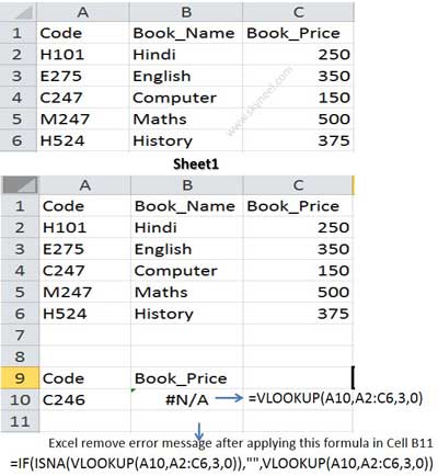
For E.g: If you have a huge database or query or table and now you want to search any values using VLookup function which is not found in selected range of cells then Excel Shows #N/A error message but you don’t want to show this error message then you have to use IF along with ISNA function in MS Excel to remove any errors which is shown during applying the formula. So, you have to take following few important steps which is given below:
Steps to Combine IF with VLookup Function to remove any errors in MS Excel:
Step 1: Create the following table on Sheet1 For E.g.:
Sheet1: A1:A6={“Code”,”H101″,”E275″,”C247″,”M247″,”H524″}
Sheet1, B1:B6={“Book_Name”,”Hindi”,”English”,”Computer”,”Maths”,”History”}
Sheet1, C1:C6={“Book_Prie”,250,350,150,500,375}
Note: After creating this table, If someone ask you if you want to find out the Book_Price for the Code 246 with the help of VLookup function in Excel, then it generate the error message #N/A in the active sheet like =VLOOKUP(A10,A2:C6,3,0). then Excel shows #N/A error message because it is not able to find the M246 code no in the range of cells Now, you want to hide this error message then you have to take few important steps which is given below:
Step 2: Take the cursor on a particular location where you want to view the result after applying the VLookup function. For E.g. type Result in the cell B11 on Sheet1.
Step 3: Now, take cursor on cell B11 and type the following given formula to CombineVLookup Function to hide any errors message in active sheet of MS Excel:
=IF(ISNA(VLOOKUP(A10,A2:C6,3,0)),””,VLOOKUP(A10,A2:C6,3,0))
after typing the formula press enter or return key, MS Excel does not shows you any error message it shows blank cell if Excel not found Lookup value in the given range of cells, but when you type any matched code number Excel immediately shows the result in appropriate cell.
Must Read: Use Data Validation, Naming the range and VLookup Function
hope you like this article, give your important suggestion regarding this article in the comment box and click on the like or share button to help others who are facing problem for hide the error message when using ” VLookup” function with the combination of IF and ISNA function in MS Excel. Thanks to all.
