All we know VLookup function is used for search values from left to right side in given array or table. But sometime we need to lookup any value in reverse order. In that situation you need to know how to use advance backward VLookup in reverse order in Excel? In this guide we have to discuss solution to use reverse VLookup in Excel.
There are two ways to use advance backward VLookup in reverse order in Excel. Either you can use VLookup with Choose function or Index with Match function to VLookup in reverse order in Excel. We have already discuss how to use Reverse VLookup in Excel with VLookup function in Excel. Now, we have to discuss Index and Match function to backward VLookup in reverse order in Excel.
Must Read: VLookup to find first few characters in Excel
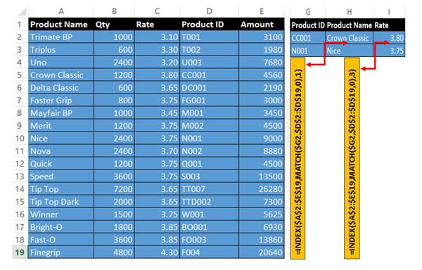
For eg: If you have an worksheet in which you have Product Name, Qty, Rate, Product ID and Amount. Now you want to lookup Product name or rate which is based on the Product ID. All we know VLookup function is used to search left to right side. But as per given condition you need to lookup value from right to left so that you must have to know how to use backward VLookup in reverse order in Excel.
Index Function in Excel
Index function return a value or the reference number to a value from given range of cells or table array.
INDEX(array, row_num, [column_num])
Array : It is a range of cells or an array constant.
Row_num : Selects the row number in an array from which to return a value. If Row_num is omitted, Column_num is required.
Column_num : It is an optional. Selects the column number in an array from which to return a value. If Column_num is omitted, Row_num is required.
Match Function in Excel
This function is used to returns the relative position of an item in the given array or range of cells that match a specific value in specific order.
MATCH (lookup value, lookup array, [match_type] )
lookup_value: The value that you want to match in lookup_array. The lookup_value argument can be any number, text, logical value or a cell reference to a number, text, or logical value.
lookup_array: It is range of cells being searched.
match_type: It is an optional. The number -1, 0, or 1. The match_type argument specifies how Excel matches lookup_value with values in lookup_array. By default value for this argument is 1.
Must Read: Advanced VLookup trick with Data Validation in Excel
Steps to use Advance Backward VLookup in Reverse Order in Excel

Step 1: Prepare the following given array table to start backward VLookup in reverse order in Excel.
Step 2: Now you want to search Product name and rate which is based on the Product ID. Product ID is placed fourth column in that situation you must have to use Index and Match function. Index and Match function allows you to use reverse VLookup in Excel.
Step 3: If you want to lookup Product name which is based on the Product ID then you have to type given formula in cell H3.
=INDEX($A$2:$E$19,MATCH($G2,$D$2:$D$19,0),1).
Step 4: If you want to search rate of product which is based on the Product ID then you have to type given formula in cell I3.
=INDEX($A$2:$E$19,MATCH($G2,$D$2:$D$19,0),3).
I hope after reading this Excel guide you can easily understand how to use Advance backward VLookup in reverse order in Excel. If you have any suggestion regarding this article then write us your suggestion in the comment box.