Conditional formatting is an important feature of Microsoft Excel. You can easily generate chess board on excel sheet with the help of excel function. In this guide we have to discuss quick way how to generate chessboard on excel with the help of conditional formatting and excel functions.
Conditional Formatting
If you want to prepare chessboard like given below on your selected range of cells in excel sheet then follow these steps given below.
Note: You can also remove conditional formatting from entire sheet or selected range of cells by clicking on the Home Tab >>> Click on the “Conditional Formatting” option in the “Styles” group >>> Click on the “Clear Rules” option > Select any required option either “Clear Rules from Selected Cells” or “Clear Rules from Entire Sheet”.
Must Read: Conditional Formatting : Only Text Entries in Excel
How to create chess board on excel:
Conditional Formatting is an important feature of Excel. This feature allow you to apply different kind of formatting on selected range of cells in active sheet. You can set background colors, borders, shading, apply styles on font that match certain given conditions.
For example if you have a large database and you want to to make a chess board on your excel sheet in that case you must follow given steps to use conditional formatting facility in excel.

Step 1: Select any range of cell in your active worksheet where you want to draw or prepare the chess board for example select the range D5:H15 > Click on the Home Tab > Click on the “Conditional Formatting” option from the “Styles” group > Click on the “New Rule” option.
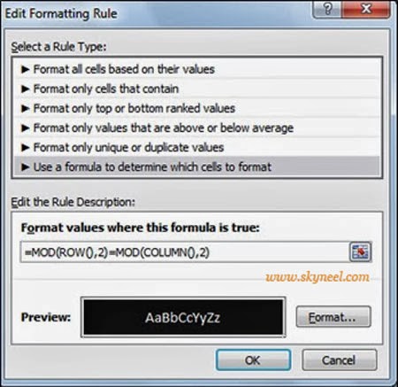
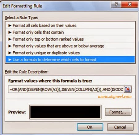
Step 2: Choose this option “Use a formula to determine which cells to format” in Select a Rule Type. Now take cursor in “Format values where this formula is true”: boxes. Type following formula to prepare chess board on excel sheet.
In this guide we have to discuss two different function which allows you to generate the chess board.
First Formula:
=MOD(ROW(),2)=MOD(COLUMN(),2)

Second Formula:
=OR(AND(ISEVEN(ROW(D5)),ISEVEN(COLUMN(D5))),AND(ISODD(ROW(D5)),ISODD(COLUMN(D5))))

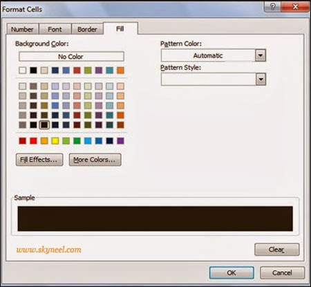
Now click on the Format button > Click on the Fill Tab > Select any background color, border or shading from format cell dialog box then click OK > Finally, click on the OK button again to make formatting on cell which match the certain given condition.

Must Read: How to find duplicates using conditional formatting in Excel
Conditional formatting is an important feature of Microsoft Excel. If you have more than one type data then easily filter data by background color or conditional formatting in active worksheet.
During working on the large worksheet, sometime you need to highlight specific cells which have specific text. There are two ways to do this job either you can do this job manually or conditional formatting. Manual method take lot of time while conditional formatting take lesser time. With the help of conditional formatting features in Excel, you can also highlight cells containing specific text.